Threshold adjacency statistics (TAS) is a technique used to extract any important information from an image. Before understanding how TAS works, let us understand thresholding in brief.
Thresholding is a technique that separates an image into a foreground region and a background region based on a specific value (threshold value). The foreground region consists of pixels whose intensity value is greater than the threshold value.
On the other hand, the background region consists of pixels whose intensity value is less than the threshold value.
TAS work by counting the number of pixels whose intensity value exceeds the threshold value. Additionally, it considers a specified number of neighboring pixels whose intensity value also exceeds the threshold value.
Threshold Adjacency Statistics in Mahotas
In Mahotas, we can use the mahotas.tas() and mahotas.pftas() functions to calculate the threshold adjacency statistics of an image. The calculated statistics can then be used to locate and extract important information from the image.
The only difference between the tas() function and the pftas() function is that in pftas() function, we can set any threshold value that is used to calculate TAS.
In contrast, the tas() function does not use a threshold value to calculate TAS.
The mahotas.tas() function
The mahotas.tas() function takes an image as input and returns a list having the threshold adjacency statistics.
Syntax
Following is the basic syntax of the tas() function in mahotas −
mahotas.features.tas(img)
where,
-
img − It is the input image.
Example
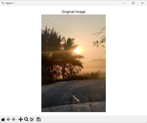
In the example mentioned below, we are calculating the TAS values of an image using the mh.tas() function.
import mahotas as mh
import numpy as np
import matplotlib.pyplot as mtplt
# Loading the images
image = mh.imread(''sun.png'')
# Computing TAS
tas = mh.features.tas(image)
# Printing the TAS value
print(tas)
# Creating a figure and axes for subplots
fig, axes = mtplt.subplots(1, 1)
# Displaying the original image
axes.imshow(image, cmap=''gray'')
axes.set_title(''Original Image'')
axes.set_axis_off()
# Adjusting spacing between subplots
mtplt.tight_layout()
# Showing the figures
mtplt.show()
Output
Output of the above code is as follows −
[8.37835351e-01 1.15467657e-02 1.39075269e-02 9.92426122e-03
1.03643093e-02  6.76089647e-03 1.09572672e-02 6.88336269e-03
8.17548510e-03  6.01115411e-02 6.08145111e-03 5.10483489e-03
4.16108390e-03  2.81568522e-03 1.77506830e-03 1.46786490e-03
6.81867008e-04  6.12677053e-04 2.44932441e-04 2.76759821e-04
. . .
4.27349413e-03  7.01932689e-03 4.50541370e-03 5.45604649e-03
6.41356563e-02  4.43892481e-03 4.80936290e-03 4.46979465e-03
3.91413752e-03  2.33898410e-03 3.27299467e-03 1.12872803e-03
2.06353013e-03  4.92334385e-04 1.22371215e-03 1.14772485e-04
6.03149199e-04  3.32444440e-05 3.26112165e-04 1.18730157e-05
1.28228570e-04  0.00000000e+00]
We get the below image as output −

The mahotas.pftas() function
The mahotas.pftas() function takes an image and a threshold value as inputs. It returns a list having the threshold adjacency statistics.
Syntax
Following is the basic syntax of the pftas() function in mahotas −
mahotas.features.pftas(img, T={mahotas.threshold.otsu(img)})
where,
-
img − It is the input image.
-
T (optional) − It defines the threshold algorithm used in TAS (by default it uses Otsu”s method).
Example
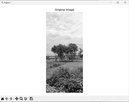
In the following example, we are computing the TAS of an image using the mh.pftas() function.
import mahotas as mh
import numpy as np
import matplotlib.pyplot as mtplt
# Loading the images
image = mh.imread(''nature.jpeg'')
# Converting it to grayscale
image = mh.colors.rgb2gray(image).astype(np.uint8)
# Computing parameter free TAS
pftas = mh.features.pftas(image)
# Printing the parameter free TAS value
print(pftas)
# Creating a figure and axes for subplots
fig, axes = mtplt.subplots(1, 1)
# Displaying the original image
axes.imshow(image, cmap=''gray'')
axes.set_title(''Original Image'')
axes.set_axis_off()
# Adjusting spacing between subplots
mtplt.tight_layout()
# Showing the figures
mtplt.show()
Output
Following is the output of the above code −
[9.57767091e-01 1.48210628e-02  8.58153775e-03  1.18217967e-02
3.89970314e-03  1.86659948e-03  7.82131473e-04  3.19863291e-04
1.40214046e-04  9.73817262e-01  1.23385295e-02  5.89271152e-03
4.39412383e-03  1.90987201e-03  8.34387151e-04  4.60922081e-04
2.31642892e-04  1.20548852e-04  9.77691695e-01  8.29460231e-03
3.91949031e-03  7.21369229e-03  1.68522833e-03  7.53014919e-04
3.10737802e-04  1.12475646e-04  1.90636688e-05  9.47186804e-01
1.14563743e-02  9.65510102e-03  1.76918166e-02  5.35205921e-03
3.38515157e-03  2.13944340e-03  1.88754119e-03  1.24570817e-03
9.80623501e-01  3.72244140e-03  2.75392589e-03  4.22681210e-03
2.28359248e-03  1.92155953e-03  1.72971300e-03  1.63378974e-03
1.10466466e-03  9.59139669e-01  7.94832237e-03  7.15439233e-03
1.68349257e-02  3.75312384e-03  1.74123294e-03  9.83390623e-04
1.06007705e-03  1.38486661e-03]
The image obtained is as follows −

Using Mean Threshold Value
We can also calculate the threshold adjacency statistics of an image using the mean threshold value. Mean threshold value refers to a threshold value calculated by taking the average pixel intensity value of an image.
In simple terms, the threshold value is calculated by adding up the intensity values of all the pixels in an image and then dividing that sum by the total number of pixels in the image.
In mahotas, we first calculate the mean threshold value using the mean() function. Then, we set this value in the T parameter of the pftas() function to calculate TAS using mean threshold value.
Example
In here, we are getting the TAS of an image using the mean threshold value.
import mahotas as mh
import numpy as np
import matplotlib.pyplot as mtplt
# Loading the images
image = mh.imread(''tree.tiff'')
# Converting it to grayscale
image = mh.colors.rgb2gray(image).astype(np.uint8)
# Calculating threshold value
threshold = image > np.mean(image)
# Computing parameter free TAS using mean threshold
pftas = mh.features.pftas(image, threshold)
# Printing the parameter free TAS value
print(pftas)
# Creating a figure and axes for subplots
fig, axes = mtplt.subplots(1, 1)
# Displaying the original image
axes.imshow(image, cmap=''gray'')
axes.set_title(''Original Image'')
axes.set_axis_off()
# Adjusting spacing between subplots
mtplt.tight_layout()
# Showing the figures
mtplt.show()
Output
After executing the above code, we get the following output −
[0.63528106  0.07587514  0.06969174 0.07046435 0.05301355 0.0396411
 0.0278772   0.0187047   0.00945114 0.51355051 0.10530301 0.0960256
 0.08990634  0.06852526  0.05097649 0.03778379 0.02519265 0.01273634
 0.69524747  0.0985423   0.07691423 0.05862548 0.03432296 0.01936853
 0.01058033  0.00482901  0.00156968 0.46277808 0.17663377 0.13243407
 0.10085554  0.06345864  0.03523172 0.01735837 0.00835911 0.00289069
 0.78372479  0.0746143   0.04885744 0.03739208 0.02555628 0.01563048
 0.00822543  0.00436208  0.00163713 0.70661663 0.07079426 0.05897885
 0.06033083  0.04280415  0.02972053 0.01632203 0.01043743 0.00399529]
The output image is as follows −
