Simple linear regression is a type of regression analysis in which a single independent variable (also known as a predictor variable) is used to predict the dependent variable. In other words, it models the linear relationship between the dependent variable and a single independent variable.

Python Implementation

Given below is an example that shows how to implement simple linear regression using the Pima-Indian-Diabetes dataset in Python. We will also plot the regression line.

Data Preparation

First, we need to import the Diabetes dataset from scikit-learn and split it into training and testing sets. We will use 80% of the data for training the model and the remaining 20% for testing.

from sklearn.datasets import load_diabetes
from sklearn.model_selection import train_test_split

# Load the Diabetes dataset
diabetes = load_diabetes()

# Split the dataset into training and testing sets
X_train, X_test, y_train, y_test = train_test_split(diabetes.data[:, 2],
diabetes.target, test_size=0.2, random_state=0)

# Reshape the input data
X_train = X_train.reshape(-1, 1)
X_test = X_test.reshape(-1, 1)

Here, we are using the third feature (column) of the dataset, which represents the mean blood pressure, as our independent variable (predictor variable) and the target variable as our dependent variable (response variable).

Model Training

We will use scikit-learn”s LinearRegression class to train a simple linear regression model on the training data. The code for this is as follows −

from sklearn.linear_model import LinearRegression
# Create a linear regression object

lr_model = LinearRegression()
# Fit the model on the training data
lr_model.fit(X_train, y_train)

Here, X_train represents the input feature (mean blood pressure) of the training data and y_train represents the output variable (target variable).

Model Testing

Once the model is trained, we can use it to make predictions on the test data. The code for this is as follows −

# Make predictions on the test data

y_pred = lr_model.predict(X_test)

Here, X_test represents the input feature of the test data and y_pred represents the predicted output variable (target variable).

Model Evaluation

We need to evaluate the performance of the model to determine its accuracy. We will use the mean squared error (MSE) and the coefficient of determination (R^2) as evaluation metrics. The code for this is as follows −

from sklearn.metrics import mean_squared_error, r2_score

# Calculate the mean squared error
mse = mean_squared_error(y_test, y_pred)

# Calculate the coefficient of determination
r2 = r2_score(y_test, y_pred)

print(''Mean Squared Error:'', mse)
print(''Coefficient of Determination:'', r2)

Here, y_test represents the actual output variable of the test data.

Plotting the Regression Line

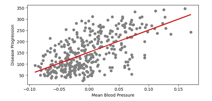
We can also visualize the regression line to see how well it fits the data. The code for this is as follows −

import matplotlib.pyplot as plt

# Plot the training data
plt.scatter(X_train, y_train, color=''gray'')

# Plot the regression line
plt.plot(X_train, lr_model.predict(X_train), color=''red'', linewidth=2)

# Add axis labels
plt.xlabel(''Mean Blood Pressure'')
plt.ylabel(''Disease Progression'')

# Show the plot
plt.show()

Here, we are using the scatter() function from the matplotlib library to plot the training data points and the plot() function to plot the regression line. The xlabel() and ylabel() functions are used to label the x-axis and y-axis of the plot, respectively. Finally, we use the show() function to display the plot.

Complete Implementation Example

The complete code for implementing simple linear regression in Python is as follows −

from sklearn.datasets import load_diabetes
from sklearn.model_selection import train_test_split
from sklearn.linear_model import LinearRegression
from sklearn.metrics import mean_squared_error, r2_score
import matplotlib.pyplot as plt

# Load the Diabetes dataset
diabetes = load_diabetes()

# Split the dataset into training and testing sets
X_train, X_test, y_train, y_test = train_test_split(diabetes.data[:, 2],
diabetes.target, test_size=0.2, random_state=0)

# Reshape the input data
X_train = X_train.reshape(-1, 1)
X_test = X_test.reshape(-1, 1)

# Create a linear regression object
lr_model = LinearRegression()

# Fit the model on the training data
lr_model.fit(X_train, y_train)

# Make predictions on the test data
y_pred = lr_model.predict(X_test)

# Calculate the mean squared error
mse = mean_squared_error(y_test, y_pred)

# Calculate the coefficient of determination
r2 = r2_score(y_test, y_pred)

print(''Mean Squared Error:'', mse)
print(''Coefficient of Determination:'', r2)

# Plot the training data
plt.figure(figsize=(7.5, 3.5))
plt.scatter(X_train, y_train, color=''gray'')

# Plot the regression line
plt.plot(X_train, lr_model.predict(X_train), color=''red'', linewidth=2)

# Add axis labels
plt.xlabel(''Mean Blood Pressure'')
plt.ylabel(''Disease Progression'')

# Show the plot
plt.show()

Output

On executing this code, you will get the following plot as the output and it will also print the Mean Squared Error and the Coefficient of Determination on the terminal −

Mean Squared Error: 4150.680189329983
Coefficient of Determination: 0.19057346847560164