Polynomial Linear Regression is a type of regression analysis in which the relationship between the independent variable and the dependent variable is modeled as an n-th degree polynomial function. Polynomial regression allows for a more complex relationship between the variables to be captured, beyond the linear relationship in Simple and Multiple Linear Regression.

Python Implementation

Here”s an example implementation of Polynomial Linear Regression using the Boston Housing dataset from Scikit-Learn −

Example

from sklearn.datasets import load_boston
from sklearn.model_selection import train_test_split
from sklearn.linear_model import LinearRegression
from sklearn.preprocessing import PolynomialFeatures
from sklearn.metrics import mean_squared_error, r2_score
import numpy as np
import matplotlib.pyplot as plt

# Load the Boston Housing dataset
boston = load_boston()

# Split the dataset into training and testing sets
X_train, X_test, y_train, y_test = train_test_split(boston.data,
boston.target, test_size=0.2, random_state=0)

# Create a polynomial features object with degree 2
poly = PolynomialFeatures(degree=2)

# Transform the input data to include polynomial features
X_train_poly = poly.fit_transform(X_train)
X_test_poly = poly.transform(X_test)

# Create a linear regression object
lr_model = LinearRegression()

# Fit the model on the training data
lr_model.fit(X_train_poly, y_train)

# Make predictions on the test data
y_pred = lr_model.predict(X_test_poly)

# Calculate the mean squared error
mse = mean_squared_error(y_test, y_pred)

# Calculate the coefficient of determination
r2 = r2_score(y_test, y_pred)

print(''Mean Squared Error:'', mse)
print(''Coefficient of Determination:'', r2)

# Sort the test data by the target variable
sort_idx = X_test[:, 12].argsort()

X_test_sorted = X_test[sort_idx]
y_test_sorted = y_test[sort_idx]

# Plot the predicted values against the actual values
plt.figure(figsize=(7.5, 3.5))
plt.scatter(y_test_sorted, y_pred[sort_idx])
plt.xlabel(''Actual Values'')
plt.ylabel(''Predicted Values'')

# Add a regression line to the plot
x = np.linspace(0, 50, 100)
y = x
plt.plot(x, y, color=''red'')

# Show the plot
plt.show()

Output

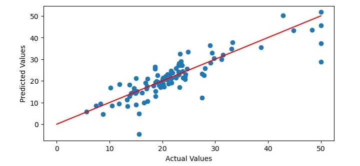
When you execute the program, it will produce the following plot as the output and it will print the Mean Squared Error and the Coefficient of Determination on the terminal −

Mean Squared Error: 25.215797617051855
Coefficient of Determination: 0.6903318065831567