Working of HDBSCAN Clustering

HDBSCAN builds a hierarchy of clusters using a mutual-reachability graph, which is a graph where each data point is a node and the edges between them are weighted by a measure of similarity or distance. The graph is built by connecting two points with an edge if their mutual reachability distance is below a given threshold.

The mutual reachability distance between two points is the maximum of their reachability distances, which is a measure of how easily one point can be reached from the other. The reachability distance between two points is defined as the maximum of their distance and the minimum density of any point along their path.

The hierarchy of clusters is then extracted from the mutual-reachability graph using a minimum spanning tree (MST) algorithm. The leaves of the MST correspond to the individual data points, while the internal nodes correspond to clusters of varying sizes and shapes.

The HDBSCAN algorithm then applies a condensed tree algorithm to the MST to extract the clusters. The condensed tree is a compact representation of the MST that only includes the internal nodes of the tree. The condensed tree is then cut at a certain level to obtain the clusters, with the level of the cut determined by a user-defined minimum cluster size or a heuristic based on the stability of the clusters.

Implementation in Python

HDBSCAN is available as a Python library that can be installed using pip. The library provides an implementation of the HDBSCAN algorithm along with several useful functions for data preprocessing and visualization.

Installation

To install HDBSCAN, open a terminal window and type the following command −

pip install hdbscan

Usage

To use HDBSCAN, first import the hdbscan library −

import hdbscan

Next, we generate a sample dataset using the make_blobs() function from scikit-learn −

# generate random dataset with 1000 samples and 3 clusters
X, y = make_blobs(n_samples=1000, centers=3, random_state=42)

Now, create an instance of the HDBSCAN class and fit it to the data −

clusterer = hdbscan.HDBSCAN(min_cluster_size=10, metric=''euclidean'')

# fit the data to the clusterer
clusterer.fit(X)

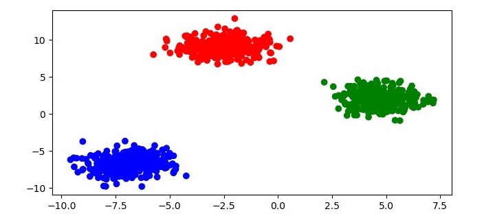
This will apply HDBSCAN to the dataset and assign each point to a cluster. To visualize the clustering results, you can plot the data with color each point according to its cluster label −

# get the cluster labels
labels = clusterer.labels_

# create a colormap for the clusters
colors = np.array([x for x in ''bgrcmykbgrcmykbgrcmykbgrcmyk''])
colors = np.hstack([colors] * 20)

# plot the data with each point colored according to its cluster label
plt.figure(figsize=(7.5, 3.5))
plt.scatter(X[:, 0], X[:, 1], c=colors[labels])
plt.show()

This code will produce a scatter plot of the data with each point colored according to its cluster label as follows −

HDBSCAN also provides several parameters that can be adjusted to fine-tune the clustering results −

• min_cluster_size − The minimum size of a cluster. Points that are not part of any cluster are labeled as noise.

• min_samples − The minimum number of samples in a neighborhood for a point to be considered a core point.

• cluster_selection_epsilon − The radius of the neighborhood used for cluster selection.

• metric − The distance metric used to measure the similarity between points.

Advantages of HDBSCAN Clustering

HDBSCAN has several advantages over other clustering algorithms −

• Better handling of clusters of varying densities − HDBSCAN can identify clusters of different densities, which is a common problem in many datasets.

• Ability to detect clusters of different shapes and sizes − HDBSCAN can identify clusters that are not necessarily spherical, which is another common problem in many datasets.

• No need to specify the number of clusters − HDBSCAN does not require the user to specify the number of clusters, which can be difficult to determine a priori.

• Robust to noise − HDBSCAN is robust to noisy data and can identify outliers as noise points.