The Decision Tree algorithm is a hierarchical tree-based algorithm that is used to classify or predict outcomes based on a set of rules. It works by splitting the data into subsets based on the values of the input features. The algorithm recursively splits the data until it reaches a point where the data in each subset belongs to the same class or has the same value for the target variable. The resulting tree is a set of decision rules that can be used to make predictions or classify new data.

The Decision Tree algorithm works by selecting the best feature to split the data at each node. The best feature is the one that provides the most information gain or the most reduction in entropy. Information gain is a measure of the amount of information gained by splitting the data at a particular feature, while entropy is a measure of the randomness or disorder in the data. The algorithm uses these measures to determine the best feature
to split the data at each node.

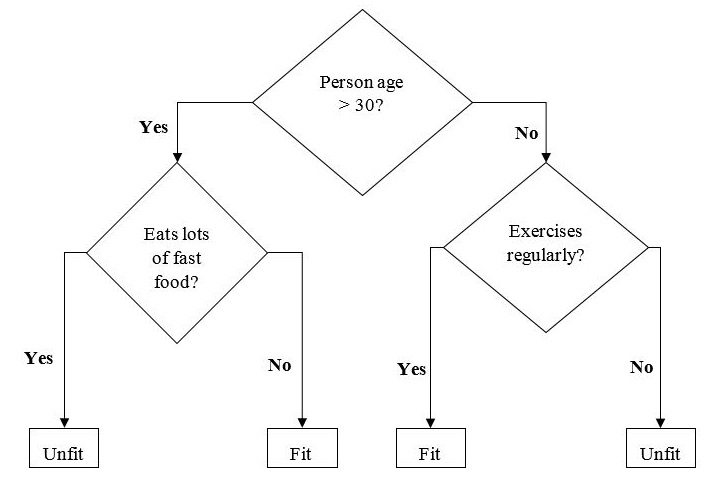
The example of a binary tree for predicting whether a person is fit or unfit providing various information like age, eating habits and exercise habits, is given below −

In the above decision tree, the question are decision nodes and final outcomes are leaves.

Types of Decision Tree Algorithm

There are two main types of Decision Tree algorithm −

• Classification Tree − A classification tree is used to classify data into different classes or categories. It works by splitting the data into subsets based on the values of the input features and assigning each subset to a different class.

• Regression Tree − A regression tree is used to predict numerical values or continuous variables. It works by splitting the data into subsets based on the values of the input features and assigning each subset a numerical value.

Implementation in Python

Let”s implement the Decision Tree algorithm in Python using a popular dataset for classification tasks named Iris dataset. It contains 150 samples of iris flowers, each with four features: sepal length, sepal width, petal length, and petal width. The flowers belong to three classes: setosa, versicolor, and virginica.

First, we will import the necessary libraries and load the dataset −

import numpy as np
from sklearn.datasets import load_iris
from sklearn.model_selection import train_test_split
from sklearn.tree import DecisionTreeClassifier

# Load the iris dataset
iris = load_iris()

# Split the dataset into training and testing sets
X_train, X_test, y_train, y_test = train_test_split(iris.data,
iris.target, test_size=0.3, random_state=0)

We then create an instance of the Decision Tree classifier and train it on the training set −

# Create a Decision Tree classifier
dtc = DecisionTreeClassifier()

# Fit the classifier to the training data
dtc.fit(X_train, y_train)

We can now use the trained classifier to make predictions on the testing set −

# Make predictions on the testing data
y_pred = dtc.predict(X_test)

We can evaluate the performance of the classifier by calculating its accuracy −

# Calculate the accuracy of the classifier
accuracy = np.sum(y_pred == y_test) / len(y_test)
print("Accuracy:", accuracy)

We can visualize the Decision Tree using Matplotlib library −

import matplotlib.pyplot as plt
from sklearn.tree import plot_tree

# Visualize the Decision Tree using Matplotlib
plt.figure(figsize=(20,10))
plot_tree(dtc, filled=True, feature_names=iris.feature_names,
class_names=iris.target_names)
plt.show()

The plot_tree function from the sklearn.tree module can be used to plot the Decision Tree. We can pass in the trained Decision Tree classifier, the filled argument to fill the nodes with color, the feature_names argument to label the features, and the class_names argument to label the target classes. We also specify the figsize argument
to set the size of the figure and call the show function to display the plot.

Complete Implementation Example

Given below is the complete implementation example of Decision Tree Classification algorithm in python using the iris dataset −

import numpy as np
from sklearn.datasets import load_iris
from sklearn.model_selection import train_test_split
from sklearn.tree import DecisionTreeClassifier

# Load the iris dataset
iris = load_iris()

# Split the dataset into training and testing sets
X_train, X_test, y_train, y_test = train_test_split(iris.data, iris.target, test_size=0.3, random_state=0)

# Create a Decision Tree classifier
dtc = DecisionTreeClassifier()

# Fit the classifier to the training data
dtc.fit(X_train, y_train)

# Make predictions on the testing data
y_pred = dtc.predict(X_test)

# Calculate the accuracy of the classifier
accuracy = np.sum(y_pred == y_test) / len(y_test)
print("Accuracy:", accuracy)

# Visualize the Decision Tree using Matplotlib
import matplotlib.pyplot as plt
from sklearn.tree import plot_tree
plt.figure(figsize=(20,10))
plot_tree(dtc, filled=True, feature_names=iris.feature_names,
class_names=iris.target_names)
plt.show()

Output

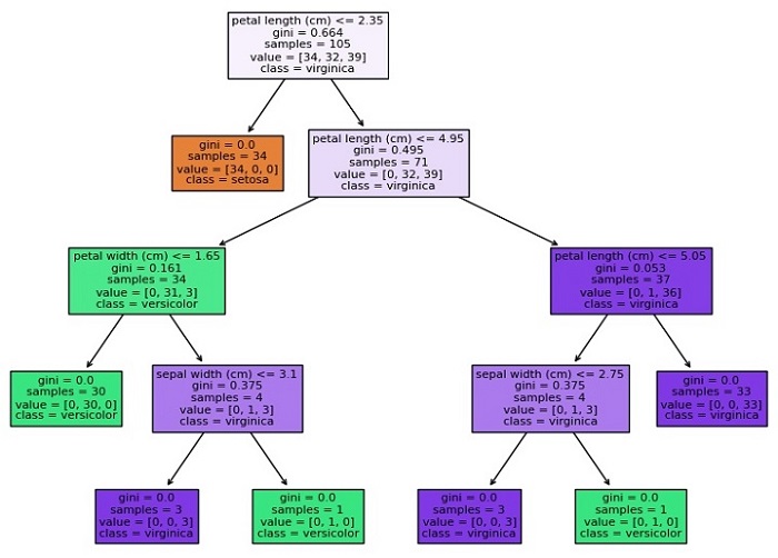
This will create a plot of the Decision Tree that looks like this −

Accuracy: 0.9777777777777777

As you can see, the plot shows the structure of the Decision Tree, with each node representing a decision based on the value of a feature, and each leaf node representing a class or numerical value. The color of each node indicates the majority class or value of the samples in that node, and the numbers at the bottom indicate the number of samples that reach that node.