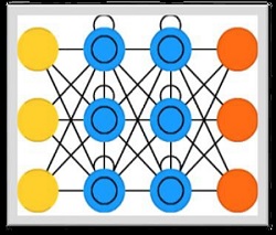
In this chapter, we will learn in detail about the sequences in CNTK and its classification.

Tensors

The concept on which CNTK works is tensor. Basically, CNTK inputs, outputs as well as parameters are organized as tensors, which is often thought of as a generalised matrix. Every tensor has a rank −

• Tensor of rank 0 is a scalar.

• Tensor of rank 1 is a vector.

• Tensor of rank 2 is amatrix.

Here, these different dimensions are referred as axes.

Static axes and Dynamic axes

As the name implies, the static axes have the same length throughout the network’s life. On the other hand, the length of dynamic axes can vary from instance to instance. In fact, their length is typically not known before each minibatch is presented.

Dynamic axes are like static axes because they also define a meaningful grouping of the numbers contained in the tensor.

Example

To make it clearer, let’s see how a minibatch of short video clips is represented in CNTK. Suppose that the resolution of video clips is all 640 * 480. And, also the clips are shot in color which is typically encoded with three channels. It further means that our minibatch has the following −

• 3 static axes of length 640, 480 and 3 respectively.

• Two dynamic axes; the length of the video and the minibatch axes.

It means that if a minibatch is having 16 videos each of which is 240 frames long, would be represented as 16*240*3*640*480 tensors.

Working with sequences in CNTK

Let us understand sequences in CNTK by first learning about Long-Short Term Memory Network.

Long-Short Term Memory Network (LSTM)

Long-short term memory (LSTMs) networks were introduced by Hochreiter & Schmidhuber. It solved the problem of getting a basic recurrent layer to remember things for a long time. The architecture of LSTM is given above in the diagram. As we can see it has input neurons, memory cells, and output neurons. In order to combat the vanishing gradient problem, Long-short term memory networks use an explicit memory cell (stores the previous values) and the following gates −

• Forget gate − As the name implies, it tells the memory cell to forget the previous values. The memory cell stores the values until the gate i.e. ‘forget gate’ tells it to forget them.

• Input gate − As name implies, it adds new stuff to the cell.

• Output gate − As name implies, output gate decides when to pass along the vectors from the cell to the next hidden state.

It is very easy to work with sequences in CNTK. Let’s see it with the help of following example −

import sys
import os
from cntk import Trainer, Axis
from cntk.io import MinibatchSource, CTFDeserializer, StreamDef, StreamDefs,
   INFINITELY_REPEAT
from cntk.learners import sgd, learning_parameter_schedule_per_sample
from cntk import input_variable, cross_entropy_with_softmax, 
   classification_error, sequence
from cntk.logging import ProgressPrinter
from cntk.layers import Sequential, Embedding, Recurrence, LSTM, Dense
def create_reader(path, is_training, input_dim, label_dim):
   return MinibatchSource(CTFDeserializer(path, StreamDefs(
      features=StreamDef(field=''x'', shape=input_dim, is_sparse=True),
      labels=StreamDef(field=''y'', shape=label_dim, is_sparse=False)
   )), randomize=is_training,
   max_sweeps=INFINITELY_REPEAT if is_training else 1)
def LSTM_sequence_classifier_net(input, num_output_classes, embedding_dim,
LSTM_dim, cell_dim):
   lstm_classifier = Sequential([Embedding(embedding_dim),
      Recurrence(LSTM(LSTM_dim, cell_dim)),
      sequence.last,
      Dense(num_output_classes)])
return lstm_classifier(input)
def train_sequence_classifier():
   input_dim = 2000
   cell_dim = 25
   hidden_dim = 25
   embedding_dim = 50
   num_output_classes = 5
   features = sequence.input_variable(shape=input_dim, is_sparse=True)
   label = input_variable(num_output_classes)
   classifier_output = LSTM_sequence_classifier_net(
   features, num_output_classes, embedding_dim, hidden_dim, cell_dim)
   ce = cross_entropy_with_softmax(classifier_output, label)
   pe =      classification_error(classifier_output, label)
   rel_path = ("../../../Tests/EndToEndTests/Text/" +
      "SequenceClassification/Data/Train.ctf")
   path = os.path.join(os.path.dirname(os.path.abspath(__file__)), rel_path)
   reader = create_reader(path, True, input_dim, num_output_classes)
input_map = {
   features: reader.streams.features,
   label: reader.streams.labels
}
lr_per_sample = learning_parameter_schedule_per_sample(0.0005)
progress_printer = ProgressPrinter(0)
trainer = Trainer(classifier_output, (ce, pe),
sgd(classifier_output.parameters, lr=lr_per_sample),progress_printer)
minibatch_size = 200
for i in range(255):
   mb = reader.next_minibatch(minibatch_size, input_map=input_map)
trainer.train_minibatch(mb)
   evaluation_average = float(trainer.previous_minibatch_evaluation_average)
   loss_average = float(trainer.previous_minibatch_loss_average)
return evaluation_average, loss_average
if __name__ == ''__main__'':
   error, _ = train_sequence_classifier()
   print(" error: %f" % error)

average  since  average  since  examples
loss     last   metric   last
------------------------------------------------------
1.61    1.61    0.886     0.886     44
1.61     1.6    0.714     0.629    133
 1.6    1.59     0.56     0.448    316
1.57    1.55    0.479      0.41    682
1.53     1.5    0.464     0.449   1379
1.46     1.4    0.453     0.441   2813
1.37    1.28     0.45     0.447   5679
 1.3    1.23    0.448     0.447  11365

error: 0.333333

The detailed explanation of the above program will be covered in next sections, especially when we will be constructing Recurrent Neural networks.