A histogram is a bar graph-like representation of the distribution of a variable. It shows the frequency of occurrences of each value of the variable. The x-axis represents the range of values of the variable, and the y-axis represents the frequency or count of each value. The height of each bar represents the number of data points that fall within that value range.

Histograms are useful for identifying patterns in data, such as skewness, modality, and outliers. Skewness refers to the degree of asymmetry in the distribution of the variable. Modality refers to the number of peaks in the distribution. Outliers are data points that fall outside of the range of typical values for the variable.

Python Implementation of Histograms

Python provides several libraries for data visualization, such as Matplotlib, Seaborn, Plotly, and Bokeh. For the example given below, we will use Matplotlib to implement histograms.

We will use the breast cancer dataset from the Sklearn library for this example. The breast cancer dataset contains information about the characteristics of breast cancer cells and whether they are malignant or benign. The dataset has 30 features and 569 samples.

Example

Let”s start by importing the necessary libraries and loading the dataset −

import matplotlib.pyplot as plt
from sklearn.datasets import load_breast_cancer
data = load_breast_cancer()

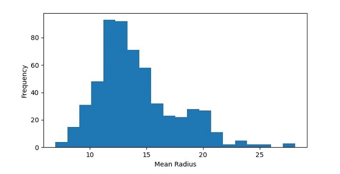
Next, we will create a histogram of the mean radius feature of the dataset −

plt.figure(figsize=(7.2, 3.5))
plt.hist(data.data[:,0], bins=20)
plt.xlabel(''Mean Radius'')
plt.ylabel(''Frequency'')
plt.show()

In this code, we have used the hist() function from Matplotlib to create a histogram of the mean radius feature of the dataset. We have set the number of bins to 20 to divide the data range into 20 intervals. We have also added labels to the x and y axes using the xlabel() and ylabel() functions.

Output

The resulting histogram shows the distribution of mean radius values in the dataset. We can see that the data is roughly normally distributed, with a peak around 12-14.

Histogram with Multiple Data Sets

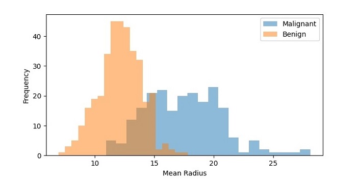
We can also create a histogram with multiple data sets to compare their distributions. Let”s create histograms of the mean radius feature for both the malignant and benign samples −

Example

plt.figure(figsize=(7.2, 3.5))
plt.hist(data.data[data.target==0,0], bins=20, alpha=0.5, label=''Malignant'')
plt.hist(data.data[data.target==1,0], bins=20, alpha=0.5, label=''Benign'')
plt.xlabel(''Mean Radius'')
plt.ylabel(''Frequency'')
plt.legend()
plt.show()

In this code, we have used the hist() function twice to create two histograms of the mean radius feature, one for the malignant samples and one for the benign samples. We have set the transparency of the bars to 0.5 using the alpha parameter so that they don”t overlap completely. We have also added a legend to the plot using the legend() function.

Output

On executing this code, you will get the following plot as the output −

The resulting histogram shows the distribution of mean radius values for both the malignant and benign samples. We can see that the distributions are different, with the malignant samples having a higher frequency of higher mean radius values.