For a stationary time series, a moving average model sees the value of a variable at time ‘t’ as a linear function of residual errors from ‘q’ time steps preceding it. The residual error is calculated by comparing the value at the time ‘t’ to moving average of the values preceding.

Mathematically it can be written as −

$$y_{t} = c:+:epsilon_{t}:+:theta_{1}:epsilon_{t-1}:+:theta_{2}:epsilon_{t-2}:+:…+:theta_{q}:epsilon_{t-q}:$$

Where‘q’ is the moving-average trend parameter

$epsilon_{t}$ is white noise, and

$epsilon_{t-1}, epsilon_{t-2}…epsilon_{t-q}$ are the error terms at previous time periods.

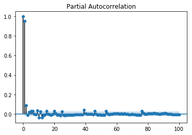
Value of ‘q’ can be calibrated using various methods. One way of finding the apt value of ‘q’ is plotting the partial auto-correlation plot.

A partial auto-correlation plot shows the relation of a variable with itself at prior time steps with indirect correlations removed, unlike auto-correlation plot which shows direct as well as indirect correlations, let’s see how it looks like for ‘temperature’ variable of our data.

Showing PACP

In [143]:

from statsmodels.graphics.tsaplots import plot_pacf

plot_pacf(train, lags = 100)
plt.show()

A partial auto-correlation is read in the same way as a correlogram.