Highlighting image maxima refers to displaying the brightest areas of an image. Image maxima, also known as regional maxima, is the area having the highest pixel intensity value amongst all other areas of an image.

The image maxima consider the entire image when searching for the brightest areas. An image can have multiple regional maxima, but all of them will have the same level of brightness. This is because only the brightest value is considered as the image maxima.

Highlighting Image Maxima in Mahotas

In Mahotas, we can use the mahotas.regmax() function to highlight maxima in an image. Image maxima represent high intensity regions; hence they are identified by looking at an image”s intensity peaks. Following is the basic approach used by the function to highlight the image maxima −

• First, it compares the intensity value of each local maxima region to its neighbors.

• If a brighter neighbor is found, the function sets it to be the new image maxima.

This process continues until all the regions have been compared to the image maxima.

The mahotas.regmax() function

The mahotas.regmax() function takes a grayscale image as input. It returns an image where the 1s represent the image maxima points, while the 0s represent normal points.

Syntax

Following is the basic syntax of the regmax() function in mahotas −

mahotas.regmax(f, Bc={3x3 cross}, out={np.empty(f.shape, bool)})

Where,

• f − It is the input grayscale image.

• Bc (optional) − It is the structuring element used for connectivity.

• out(optional) − It is the output array of Boolean data type (defaults to new array of same size as f).

Example

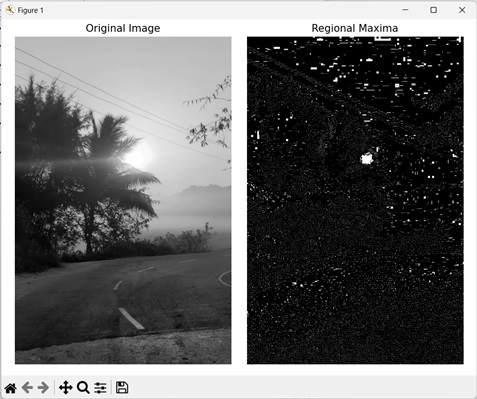
In the following example, we are highlighting image maxima using the mh.regmax() function.

import mahotas as mh
import numpy as np
import matplotlib.pyplot as mtplt
# Loading the image
image = mh.imread(''sun.png'')
# Converting it to grayscale
image = mh.colors.rgb2gray(image)
# Getting the regional maxima
regional_maxima = mh.regmax(image)
# Creating a figure and axes for subplots
fig, axes = mtplt.subplots(1, 2)
# Displaying the original image
axes[0].imshow(image, cmap=''gray'')
axes[0].set_title(''Original Image'')
axes[0].set_axis_off()
# Displaying the highlighted image maxima
axes[1].imshow(regional_maxima, cmap=''gray'')
axes[1].set_title(''Regional Maxima'')
axes[1].set_axis_off()
# Adjusting spacing between subplots
mtplt.tight_layout()
# Showing the figures
mtplt.show()

Output

Following is the output of the above code −

Highlighting Maxima by using custom Structuring Element

We can also highlight the image maxima by using a custom structuring element. A structuring element is an array consisting of only ones and zeroes. It defines the connectivity pattern of the neighborhood pixels.

Pixels with the value 1 are included in connectivity analysis while the pixels with the value 0 are excluded.

In mahotas, we create a custom structuring element using the mh.disk() function. Then, we set this custom structuring element as the Bc parameter in the regmax() function to highlight the image maxima.

Example

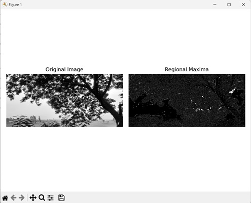
In this example, we are highlighting the image maxima by using a custom structuring element.

import mahotas as mh
import numpy as np
import matplotlib.pyplot as mtplt
# Loading the image
image = mh.imread(''tree.tiff'')
# Converting it to grayscale
image = mh.colors.rgb2gray(image)
# Creating a custom structuring element
se = np.array([[0, 1, 0],[1, 1, 1],[0, 1, 0]])
# Getting the regional maxima
regional_maxima = mh.regmax(image, Bc=se)
# Creating a figure and axes for subplots
fig, axes = mtplt.subplots(1, 2)
# Displaying the original image
axes[0].imshow(image, cmap=''gray'')
axes[0].set_title(''Original Image'')
axes[0].set_axis_off()
# Displaying the highlighted image maxima
axes[1].imshow(regional_maxima, cmap=''gray'')
axes[1].set_title(''Regional Maxima'')
axes[1].set_axis_off()
# Adjusting spacing between subplots
mtplt.tight_layout()
# Showing the figures
mtplt.show()

Output

After executing the above code, we get the following output −